Introduction to Gaussian Processes
[1]:
# © Crown Copyright GCHQ
#
# Licensed under the GNU General Public License, version 3 (the "License");
# you may not use this file except in compliance with the License.
# You may obtain a copy of the License at
#
# https://www.gnu.org/licenses/gpl-3.0.en.html
#
# Unless required by applicable law or agreed to in writing, software
# distributed under the License is distributed on an "AS IS" BASIS,
# WITHOUT WARRANTIES OR CONDITIONS OF ANY KIND, either express or implied.
# See the License for the specific language governing permissions and
# limitations under the License.
This notebook will introduce the theory behind Gaussian processes, and showcase some of the implementations of them in Python.
[2]:
random_seed = 1_989
[3]:
import gpytorch
import matplotlib.pyplot as plt
import numpy as np
import torch
from numpy.typing import NDArray
from sklearn.gaussian_process import GaussianProcessRegressor
from sklearn.gaussian_process.kernels import RBF, ConstantKernel
from torch import Tensor
from typing_extensions import override

from vanguard.datasets.synthetic import SyntheticDataset, very_complicated_f
from vanguard.kernels import ScaledRBFKernel
from vanguard.vanilla import GaussianGPController
Regression
Suppose we have some data made up of input (\(x\)) and output (\(y\)) values, and we wish to fit a model which will allow us to predict new outputs in future. This is a regression problem, and our model takes the form of the function \(f\) in the following equation:
where we assume that \(\epsilon_i\sim N(0, \sigma_i^2)\). In linear regression, we might assume that \(f\) is of the form:
We can often get a better fit by including more terms, adding an \(x_i^2\) coefficient and so on, but this still has its limits. In fact, we can add many complex terms in an attempt to make our model as general as possible, but this becomes complicated and is ultimately very fragile. Being Bayesian, we want to place priors over our unknowns and infer posteriors using the data.
Gaussian Processes
Gaussian processes (GPs) provide the probability distribution we require over functions. “Gaussian” refers to the fact that values at any point follow some normal distribution, to be inferred. GP regression is extremely flexible as one’s assumptions about the unknown function \(f\) are at a higher level of abstraction than in other methods.
Having determined the posterior, you can obtain predictions for \(f(x)\) at any collection of \(x\) values. These predictions are not just point estimates but full probability distributions, meaning that confidence estimates can be obtained. For any input you receive not just the prediction, but a measure of how sure the model is about that prediction.
To summarise, the main advantages of GP regression models are:
Observation uncertainty on \(y\)-values is quantified. If you are unsure about your true \(y\)-values to begin with, then the GP will take this into account.
Extrapolation uncertainty is quantified. The further away the point you wish to predict is from truth data, the less sure your model will be about its prediction.
Flexible posteriors, allowing you to include more upfront information about the expected behaviour of the model.
Predictions come with full probability distributions for uncertainty quantification.
Theoretical Shortcomings
Standard GP regression is not a panacea for regression problems, and one should take the following into account:
Predictions must be normally distributed, which may be at odds with what you know about the data (e.g., always positive).
Uncertainty on the input (\(x\)) values cannot be handled, meaning that the model may be more sure about a prediction than it ought to be.
Exact inference scales cubically with dataset size. This means that for \(n\) data points, the inference runs in \(\mathcal{O}(n^3)\) time, which can get very slow very quickly.
The Mathematics Behind Gaussian Processes
Gaussian processes are not an easy thing to understand, and the allusion to linear and multinomial regression can only carry the reader so far. The following explanation is taken from Chapter 2 of [Rasmussen06], which although a thorough exploration of the theory, does not make for light reading.
A Gaussian process is completely specified by its mean function and covariance function. These are denoted by \(m(x)\) and \(k(x, x')\) respectively, and defined as follows:
Note that the covariance between the outputs is written as a function of the inputs. We write the Gaussian process as a distribution not dissimilar to a Gaussian distribution, except instead of being over the real numbers it is over the function space over the reals:
A common choice for the mean function is the zero function:
and a common choice for the covariance function is the squared exponential function:
(Other choices are available, and when to use them depends on the type of data you have, and behaviours you expect from your model.) As the distance between \(x\) and \(x'\) decreases to zero, the covariance approaches 1, and as the distance increases to infinity, the covariance approaches zero. This makes sense, since the effect of a given data point on our truth data should depend somewhat on how close we are to that data point.
In order to understand the mathematics, it helps to consider the case where we have a zero mean, and there is no noise on the observations, i.e. the training data we have is exact with no uncertainty on the \(y\)-values. Consider the model \(f\) we fit over the \(n\) observations (our training data) not as a function per se, but as a distribution from which we draw said function. Suppose we wish to predict the \(y\)-values over \(n_*\) test data points, then the joint distribution of the training outputs (\(f\)) and the test outputs (\(f*\)) with respect to the prior is:
where \(K(X,X_*)\) denotes the \(n\times n_*\) matrix of the covariances calculated at all pairs of training and test points (subject to our covariance function \(k\)), and similar for all other \(K(\cdot,\cdot)\). To infer the posterior distribution we also restrict this joint prior distribution to function which will concur with the observations. We do this by conditioning the joint prior on the observations using standard Gaussian conditioning rules, which gives the following formula for our \(f_*\) distribution:
where
Function values can then be sampled from this distribution, which will yield our model for the test values. This is how prediction works for a Gaussian process, and explains the uncertainty that the model includes with it. Note the required inverse of the \(K(X, X)\) matrix, which explains the cubic complexity of the inference.
Python Implementations of GPs
Many data science and machine learning libraries exist which can implement simple Gaussian processes. The data we will
be using is the SyntheticDataset, with the
vanguard.datasets.synthetic.very_complicated_f() function, given by:
[4]:
DATASET = SyntheticDataset(functions=[very_complicated_f], n_train_points=10, rng=np.random.default_rng(random_seed))
Sci-kit Learn
The most straightforward implementation is in sklearn, with a trademark light-weight API. We first need a kernel,
which is the Python equivalent which implements the covariance function \(k\). The
RBF kernel is the implementation of the squared exponential covariance
function mentioned above. We compose it with a ConstantKernel, to allow us to
scale the covariance to accommodate the prior:
[5]:
kernel = ConstantKernel() * RBF()
We can then instantiate our model with the kernel:
[6]:
gp = GaussianProcessRegressor(kernel=kernel, n_restarts_optimizer=9, alpha=DATASET.train_y_std.detach().cpu().numpy())
As is common with sklearn we call the fit() method, which
will tune the hyperparameters in the mean and the kernel of the Gaussian process:
[7]:
gp.fit(DATASET.train_x.detach().cpu().numpy(), DATASET.train_y.detach().cpu().numpy())
[7]:
GaussianProcessRegressor(alpha=array(0.1, dtype=float32),
                         kernel=1**2 * RBF(length_scale=1),
                         n_restarts_optimizer=9)
In a Jupyter environment, please rerun this cell to show the HTML representation or trust the notebook. On GitHub, the HTML representation is unable to render, please try loading this page with nbviewer.org.
Parameters
| kernel | 1**2 * RBF(length_scale=1) | |
| alpha | array(0.1, dtype=float32) | |
| optimizer | 'fmin_l_bfgs_b' | |
| n_restarts_optimizer | 9 | |
| normalize_y | False | |
| copy_X_train | True | |
| n_targets | None | |
| random_state | None | |
| kernel__k1 | 1**2 | |
| kernel__k2 | RBF(length_scale=1) | |
| kernel__k1__constant_value | 1.0 | |
| kernel__k1__constant_value_bounds | (1e-05, ...) | |
| kernel__k2__length_scale | 1.0 | |
| kernel__k2__length_scale_bounds | (1e-05, ...) |
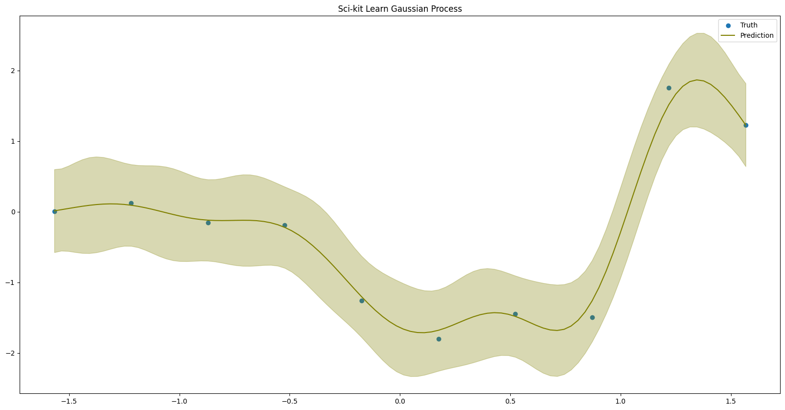
Our predictions can then be pulled from the model using the
predict() method. By predicting across a mesh of points over
the training data, we can see the effects of the uncertainty on the plot.
[8]:
linspace = np.linspace(DATASET.train_x.min().item(), DATASET.train_x.max().item(), num=100)
predictions, uncertainty = gp.predict(linspace.reshape(-1, 1), return_std=True)
[9]:
# Convert to numpy arrays for plotting
plt_train_x = DATASET.train_x.numpy(force=True)
plt_train_y = DATASET.train_y.numpy(force=True)

plt.figure(figsize=(20, 10))
plt.scatter(plt_train_x, plt_train_y, label="Truth")
plt.plot(linspace, predictions, color="olive", label="Prediction")
plt.fill_between(linspace, predictions - 1.96 * uncertainty, predictions + 1.96 * uncertainty, color="olive", alpha=0.3)
plt.title("Sci-kit Learn Gaussian Process")
plt.legend()
plt.show()
GPyTorch
Sci-kit learn is a great choice for implementing a quick GP, but it has very little room for adjustment and it is almost
impossible to do anything advanced. On the other side of the spectrum, gpytorch allows for an almost unbounded set
of features by fully exposing all parts of the GP architecture. Our initial kernel is identical to the above example,
composing the RBFKernel with a ScaleKernel:
[10]:
kernel = gpytorch.kernels.ScaleKernel(gpytorch.kernels.RBFKernel())
We also now have freedom over the mean. A good starting place is the ConstantMean:
[11]:
mean = gpytorch.means.ConstantMean()
Unlike sklearn, we need to specify a likelihood function, which controls the mapping from the image of points under
a function (\(f(x)\)) to the labels. This can be as simple as adding some Gaussian noise as in the
GaussianLikelihood, or something more complex to enable binary classification as in the
BernoulliLikelihood. However, the former is the best choice for a simple model:
[12]:
likelihood = gpytorch.likelihoods.GaussianLikelihood()
Finally, we need to build a model class to handle the inference. GPyTorch makes you do this yourself to allow you full
control, but it can seem like a daunting task. For a simple case, one need only subclass the
ExactGP class, and specify a forward method to pass data through the mean and covariance
functions. The MultivariateNormal instance is the standard output for these functions,
allowing us to work with a distribution directly instead of separating the mean and variance.
[13]:
class ExactGPModel(gpytorch.models.ExactGP):
    def __init__(self, train_x: Tensor, train_y: Tensor, y_std: Tensor) -> None:
        likelihood = gpytorch.likelihoods.FixedNoiseGaussianLikelihood(noise=y_std)
        super().__init__(train_x, train_y, likelihood)
        self.mean_module = gpytorch.means.ConstantMean()
        self.covar_module = gpytorch.kernels.ScaleKernel(gpytorch.kernels.RBFKernel())

    @override
    def forward(self, x: Tensor) -> gpytorch.distributions.MultivariateNormal:
        mean_x = self.mean_module(x)
        covar_x = self.covar_module(x)
        return gpytorch.distributions.MultivariateNormal(mean_x, covar_x)
We can then instantiate our model. Note that GPyTorch works with tensors instead of numpy arrays, so we need to ensure that we convert them before passing them to the model.
[14]:
gp = ExactGPModel(
    torch.as_tensor(DATASET.train_x),
    torch.as_tensor(DATASET.train_y),
    torch.ones(len(DATASET.train_y)) * DATASET.train_y_std,
)
Fitting the model is a much more manual task here than it was before, requiring us to build our own function. We make
use of the Adam optimiser, and also the ExactMarginalLogLikelihood class.
This will compute the marginal log likelihood of the model when applied to some data, and can be turned into “loss”
functions by negating them. There are a few variations, but this one is sufficient for this simple case. We wrap all of
these into a fit function to broadly emulate the one from sklearn:
[15]:
optimiser = torch.optim.Adam([{"params": gp.parameters()}], lr=0.1)
mll = gpytorch.mlls.ExactMarginalLogLikelihood(gp.likelihood, gp)


def fit(model: ExactGPModel, train_x: Tensor, train_y: Tensor, n_iters: int) -> None:
    model.train()
    model.likelihood.train()

    for i in range(n_iters):
        optimiser.zero_grad()
        output = model(train_x)
        loss = -mll(output, train_y)
        loss.backward()
        optimiser.step()
[16]:
fit(gp, torch.as_tensor(DATASET.train_x), torch.as_tensor(DATASET.train_y), n_iters=100)
Again, we are expected to craft our own predict method, which is much simpler:
[17]:
def predict(model: ExactGPModel, x: Tensor) -> tuple[NDArray[float], NDArray[float]]:
    model.eval()
    model.likelihood.eval()

    with torch.no_grad(), gpytorch.settings.fast_pred_var():
        prediction = model.likelihood(model(x))

    means = prediction.loc.numpy(force=True)
    variances = prediction.lazy_covariance_matrix.diagonal().numpy(force=True)

    return means, np.sqrt(np.abs(variances))
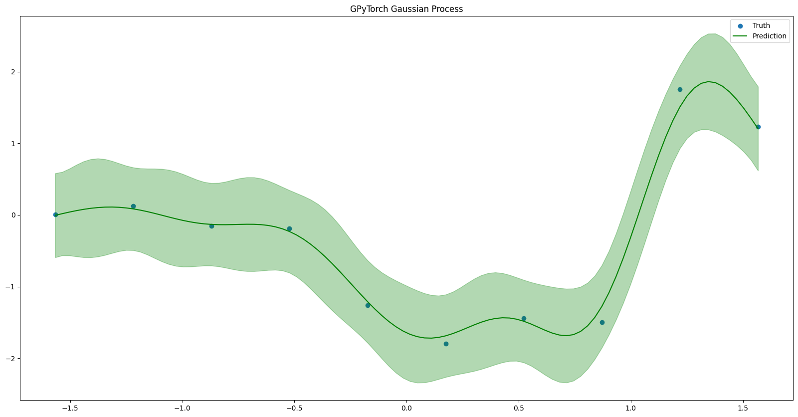
As before, we can see how well the model incorporates uncertainty:
[18]:
predictions, uncertainty = predict(gp, torch.as_tensor(linspace))
/home/docs/checkouts/readthedocs.org/user_builds/vanguard/envs/latest/lib/python3.13/site-packages/gpytorch/likelihoods/gaussian_likelihood.py:347: GPInputWarning: You have passed data through a FixedNoiseGaussianLikelihood that did not match the size of the fixed noise, *and* you did not specify noise. This is treated as a no-op.
  warnings.warn(
[19]:
plt.figure(figsize=(20, 10))
plt.scatter(plt_train_x, plt_train_y, label="Truth")
plt.plot(linspace, predictions, color="green", label="Prediction")
plt.fill_between(linspace, predictions - 1.96 * uncertainty, predictions + 1.96 * uncertainty, color="green", alpha=0.3)
plt.title("GPyTorch Gaussian Process")
plt.legend()
plt.show()
Vanguard
Finally, we come to Vanguard, which is built upon GPyTorch to allow advanced GP functionality without requiring too much
knowledge from the user. Given its base, Vanguard can be adjusted to use many components from GPyTorch, and also allows
for easy composability of the advanced features made available. Instead of composing our own kernels (which is still
possible) we use the specific ScaledRBFKernel. Note that components are passed around in
Vanguard as uninstantiated classes instead of instances, which enables much of the composability.
[20]:
gp = GaussianGPController(
    DATASET.train_x,
    DATASET.train_y,
    kernel_class=ScaledRBFKernel,
    y_std=DATASET.train_y_std,
    rng=np.random.default_rng(random_seed),
)
gp.fit(100)
/home/docs/checkouts/readthedocs.org/user_builds/vanguard/envs/latest/lib/python3.13/site-packages/torch/utils/_device.py:104: UserWarning: To copy construct from a tensor, it is recommended to use sourceTensor.detach().clone() or sourceTensor.detach().clone().requires_grad_(True), rather than torch.tensor(sourceTensor).
  return func(*args, **kwargs)
/home/docs/checkouts/readthedocs.org/user_builds/vanguard/envs/latest/lib/python3.13/site-packages/vanguard/base/basecontroller.py:573: UserWarning: A regression problem with no warping may suffer from numerical instability in optimisation if the y values are not standard scaled. Using the NormaliseY decorator will likely help.
  warnings.warn(
[20]:
tensor(1.4409)
Instead of a predict method, Vanguard opts for the
posterior_over_point() method, which will return an instance of a
Posterior class, allowing some of the features to alter how the distribution leads to
predictions.
[21]:
posterior = gp.predictive_likelihood(linspace)
predictions, covar = posterior._tensor_prediction()
predictions, covar = predictions.numpy(force=True), covar.numpy(force=True)
uncertainty = np.sqrt(covar.diagonal())
To simplify matters, one can just call the confidence_interval() method
instead of working directly with the covariance matrix:
[22]:
median, lower, upper = posterior.confidence_interval()

# Convert to numpy for plotting
median = median.numpy(force=True)
lower = lower.numpy(force=True)
upper = upper.numpy(force=True)

plt.figure(figsize=(20, 10))
plt.scatter(plt_train_x, plt_train_y, label="Truth")
plt.plot(linspace, median, color="red", label="Prediction")
plt.fill_between(linspace, lower, upper, color="red", alpha=0.3)
plt.title("Vanguard Gaussian Process")
plt.legend()
plt.show()
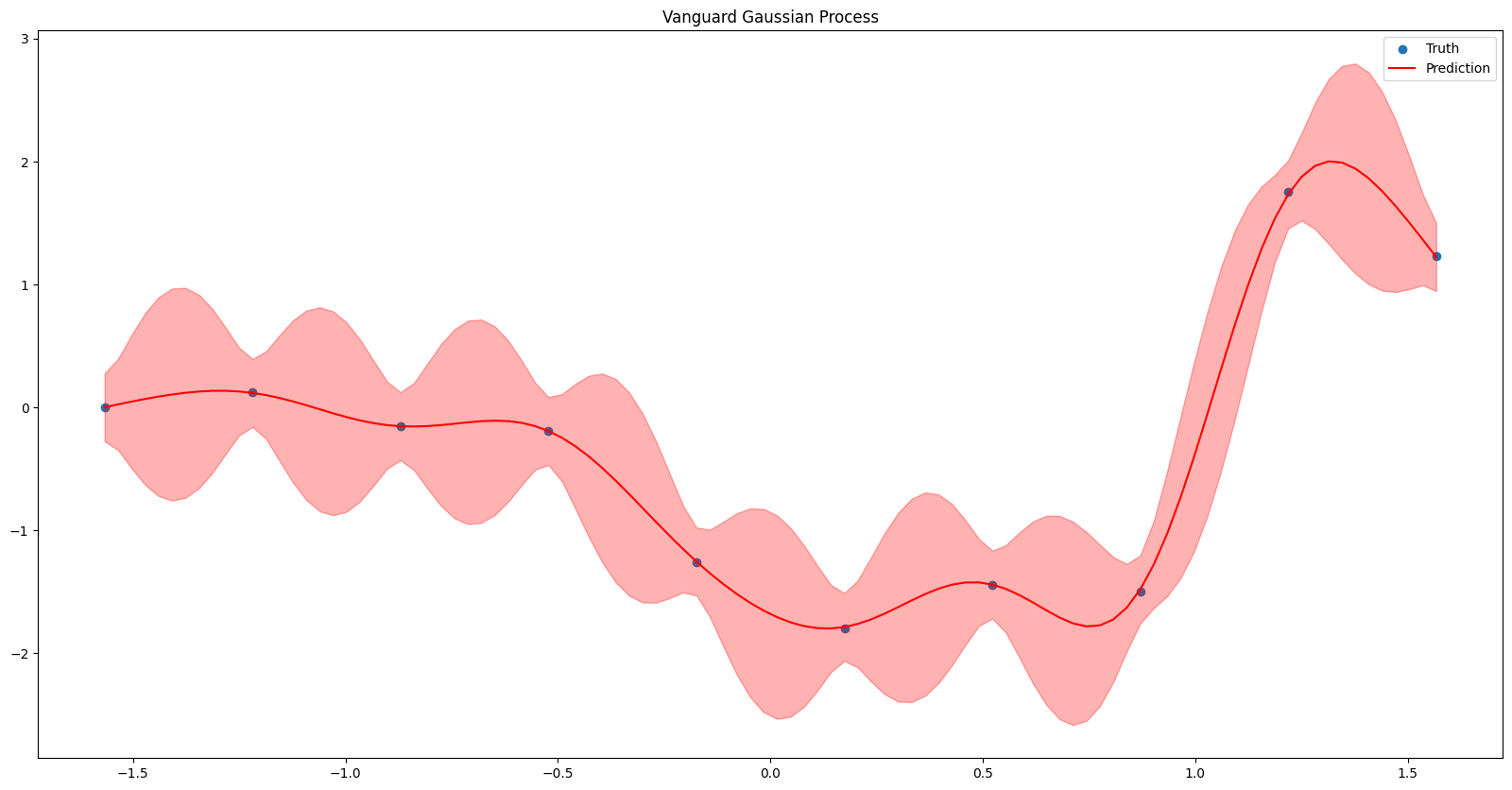
This is arguably the best fit, as the uncertainty around the target values is properly accounted for, yet the mean still follows the overall trend of the points. Vanguard also scales its inputs by default, which often leads to faster convergence.
Conclusions
In this notebook we have introduced the theory of Gaussian processes, and compared some common Python implementations. In order to see how advanced features can be applied using Vanguard, have a look through some other example notebooks for specific examples.